We designed this package to provide several functions for area-level
small area estimation under Spatial Simultaneous Autoregressive (SAR)
and Leroux Conditional Autoregressive (CAR) models, accommodating survey
design effect (DEFF) adjustments, using hierarchical Bayesian (HB)
method with Beta distribution for variables of interest. Some datasets
simulated by a data generation are also provided. The rjags
package is employed to obtain parameter estimates using Gibbs Sampling
algorithm. Model-based estimators involve the HB estimators which
include the mean estimation, the estimated model coefficients, the
random effect, and the random effect variance. For the reference, see
Rao and Molina (2015), Kubacki and Jedrzejczak (2016), Leroux et
al. (2000), and Chung and Datta (2020).
Boby Iwan, Cucu Sumarni
Boby Iwan bobyiwanboby2122@gmail.com
betadeff_sar() Estimates small area means using a
Spatial SAR Model under a Beta distribution, incorporating survey design
effect (DEFF) adjustments.beta_sar() Estimates small area means using a Spatial
SAR Model under a Beta distribution without DEFF adjustments, by
estimating the unknown precision parameter.betadeff_lerouxcar() Estimates small area means using a
Spatial Leroux CAR Model under a Beta distribution, incorporating survey
design effect (DEFF) adjustments.beta_lerouxcar() Estimates small area means using a
Spatial Leroux CAR Model under a Beta distribution without DEFF
adjustments, by estimating the unknown precision parameter.betadeff_nonspatial() Estimates small area means using
a Non-Spatial Model under a Beta distribution with Independent and
Identically Distributed (IID) random effects, incorporating DEFF
adjustments.beta_nonspatial() Estimates small area means using a
Non-Spatial Model under a Beta distribution with IID random effects
without DEFF adjustments, by estimating the unknown precision
parameter.build_w() A utility function to construct spatial
weights matrices (contiguity, distance, or kernel) required for spatial
modeling.moran_test() A diagnostic function to perform Moran’s I
test for spatial autocorrelation.You can install the development version of saeHB.Spatial.Beta from GitHub with:
# install.packages("devtools")
devtools::install_github("BobyIwan/saeHB.Spatial.Beta")
Or, to include the vignette:
devtools::install_github("BobyIwan/saeHB.Spatial.Beta", build_vignettes = TRUE)This is a basic example of using the betadeff_sar()
function to make an estimate based on synthetic data in this
package:
library(saeHB.Spatial.Beta)

# Load dataset and proximity matrix
data(databeta)
data(weight_mat)

# Fitting the Spatial SAR model
model_sar_deff <- betadeff_sar(
  formula = y ~ x1 + x2,
  deff = "deff",
  n_i = "n_i",
  proxmat = weight_mat,
  data = databeta
)
Extract the mean estimation for the areas:
head(model_sar_deff$est)
#>        Estimate  Est.Error   l-95% CI  u-95% CI
#> mu[1] 0.8733168 0.04930364 0.76952538 0.9521954
#> mu[2] 0.6701813 0.08491170 0.51026583 0.8503483
#> mu[3] 0.5614027 0.06997444 0.42116653 0.6891348
#> mu[4] 0.2284165 0.06585628 0.11267368 0.3603505
#> mu[5] 0.2291424 0.07970595 0.09536724 0.3880149
#> mu[6] 0.9381786 0.02863821 0.87710262 0.9851179
Extract the estimated model coefficients:
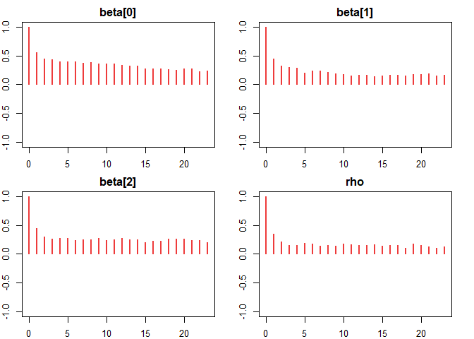
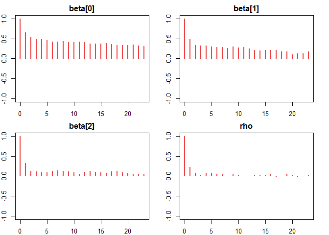
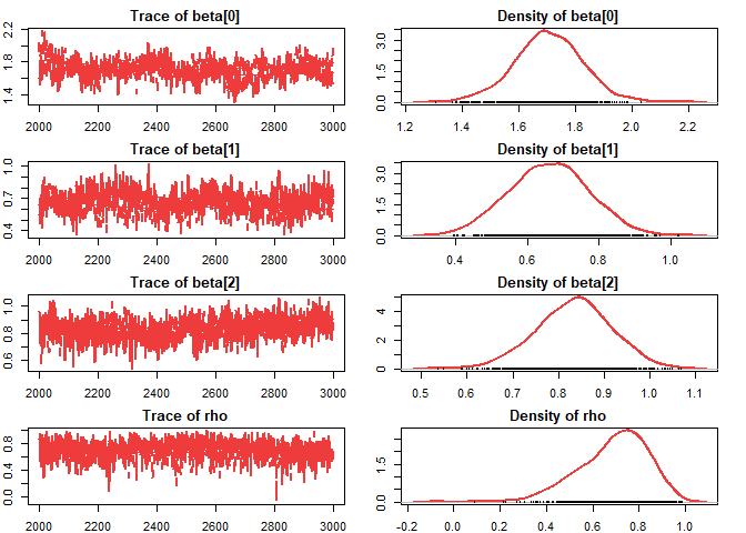
model_sar_deff$coefficient
#>          Estimate  Est.Error  l-95% CI  u-95% CI     Rhat       ESS
#> beta[0] 1.7055337 0.11951894 1.4620974 1.9419599 1.149548  66.70198
#> beta[1] 0.6605003 0.10885851 0.4504252 0.8648356 1.286895 176.22281
#> beta[2] 0.8336673 0.08175262 0.6674418 0.9867496 1.018137 237.12147
#> rho     0.6909635 0.14591695 0.3733486 0.9296335 1.124197 689.47647
Extract the random effect for the areas:
model_sar_deff$randeff
#>          Estimate Est.Error    l-95% CI   u-95% CI
#> v[1]   0.02976288 0.4913420 -0.81082629  1.0627591
#> v[2]  -0.48294515 0.4130690 -1.26231341  0.4176781
#> v[3]  -1.45769631 0.2796486 -2.00757022 -0.9495101
#> v[4]  -2.22277069 0.3881942 -3.03673421 -1.5279135
#> v[5]  -1.64869564 0.4580919 -2.58002521 -0.9115122
#> v[6]  -0.62490246 0.5151320 -1.42893550  0.6018907
#> v[7]  -1.31435972 0.3882503 -2.19447057 -0.5504201
#> v[8]  -0.59620167 0.4450396 -1.39301122  0.3173124
#> v[9]  -0.95142395 0.5666047 -1.97008703  0.1204738
#> v[10] -1.86188398 0.5945596 -2.89386412 -0.5135673
#> v[11] -0.63652811 0.5225169 -1.83768964  0.2488411
#> v[12] -0.90714526 0.6641371 -1.96549002  0.5444394
#> v[13] -0.02096918 0.4392347 -0.68315270  0.9051771
#> v[14] -0.45119582 0.3669391 -1.17877921  0.2616308
#> v[15] -0.45713340 0.3477433 -1.13515648  0.3267205
#> v[16] -0.78596192 0.4795931 -1.66931806  0.1213205
#> v[17]  0.50418771 0.6097966 -0.49833501  1.8635032
#> v[18]  0.27799928 0.5841174 -0.84562838  1.2239715
#> v[19]  1.11034886 0.3616849  0.55680893  1.9703014
#> v[20] -1.49159085 0.3551025 -2.29804991 -0.7811928
#> v[21] -1.09415346 0.6454870 -2.32510864  0.1760261
#> v[22] -0.27706199 0.3827362 -0.98308670  0.5526622
#> v[23]  0.21086216 0.5909151 -1.05375351  1.4838056
#> v[24]  1.47451757 0.6029423  0.38350864  2.9469047
#> v[25]  1.05609850 0.6278718  0.03317434  2.2172461
#> v[26]  0.33959270 0.4502330 -0.51380065  1.1474950
#> v[27]  0.14925259 0.4689303 -0.87424837  1.0693728
#> v[28]  0.22145721 0.6168820 -1.02130464  1.5324451
#> v[29]  0.96589620 0.5730657  0.07019757  2.3534697
#> v[30]  1.45079715 0.4512189  0.61843455  2.4450905
#> v[31]  0.10774431 0.6070810 -0.99013546  1.2600864
#> v[32]  0.67029354 0.9085850 -0.90793803  2.1876036
#> v[33]  1.19490972 0.5864462  0.05177372  2.3811276
#> v[34]  0.82487094 0.5193530 -0.19980381  1.7372592
#> v[35]  0.82003029 0.6997081 -0.20605962  2.5197002
#> v[36]  1.75099923 0.5749532  0.62416400  2.6853996
Extract the random effect variance for the areas:
model_sar_deff$refvar
#>           Estimate Est.Error  l-95% CI u-95% CI
#> a.var[1]  2.338106  4.781148 0.8432360 7.458702
#> a.var[2]  2.263956  4.788653 0.8277110 7.304105
#> a.var[3]  2.102129  4.732050 0.7882035 6.808402
#> a.var[4]  2.102129  4.732050 0.7882035 6.808402
#> a.var[5]  2.263956  4.788653 0.8277110 7.304105
#> a.var[6]  2.338106  4.781148 0.8432360 7.458702
#> a.var[7]  2.263956  4.788653 0.8277110 7.304105
#> a.var[8]  2.211989  4.828332 0.8111973 7.250767
#> a.var[9]  2.053250  4.772112 0.7767535 6.703232
#> a.var[10] 2.053250  4.772112 0.7767535 6.703232
#> a.var[11] 2.211989  4.828332 0.8111973 7.250767
#> a.var[12] 2.263956  4.788653 0.8277110 7.304105
#> a.var[13] 2.102129  4.732050 0.7882035 6.808402
#> a.var[14] 2.053250  4.772112 0.7767535 6.703232
#> a.var[15] 1.927767  4.732744 0.7612544 6.192884
#> a.var[16] 1.927767  4.732744 0.7612544 6.192884
#> a.var[17] 2.053250  4.772112 0.7767535 6.703232
#> a.var[18] 2.102129  4.732050 0.7882035 6.808402
#> a.var[19] 2.102129  4.732050 0.7882035 6.808402
#> a.var[20] 2.053250  4.772112 0.7767535 6.703232
#> a.var[21] 1.927767  4.732744 0.7612544 6.192884
#> a.var[22] 1.927767  4.732744 0.7612544 6.192884
#> a.var[23] 2.053250  4.772112 0.7767535 6.703232
#> a.var[24] 2.102129  4.732050 0.7882035 6.808402
#> a.var[25] 2.263956  4.788653 0.8277110 7.304105
#> a.var[26] 2.211989  4.828332 0.8111973 7.250767
#> a.var[27] 2.053250  4.772112 0.7767535 6.703232
#> a.var[28] 2.053250  4.772112 0.7767535 6.703232
#> a.var[29] 2.211989  4.828332 0.8111973 7.250767
#> a.var[30] 2.263956  4.788653 0.8277110 7.304105
#> a.var[31] 2.338106  4.781148 0.8432360 7.458702
#> a.var[32] 2.263956  4.788653 0.8277110 7.304105
#> a.var[33] 2.102129  4.732050 0.7882035 6.808402
#> a.var[34] 2.102129  4.732050 0.7882035 6.808402
#> a.var[35] 2.263956  4.788653 0.8277110 7.304105
#> a.var[36] 2.338106  4.781148 0.8432360 7.458702