ggCheysson

Version 1.1.0; documentation built 2026-09-28

The ggCheysson package brings the graphical styles of the Albums de Statistique Graphique to R and ggplot2.

The Albums were produced by the Ministry of Public Works in France under the direction of Émile Cheysson from 1879-1897. They represent the “pinnacle of the Golden Age of Statistical Graphics” (Friendly, 2008) for their innovation in visualization techniques, graphic design and beauty.

The package is based on work by:

• David Rumsey Map Collection: Complete digitized Albums de Statistique Graphique View collection
• RJ Andrews: Classic Map Color Design | GitHub
• Tom Shanley: Observable implementation Cheysson Color Palettes
• Kenneth Fields: Hand-drawn font family creation The style of Émile Cheysson

🏛️ Historical Context

The Albums de Statistique Graphique were published annually by France’s Ministry of Public Works, showcasing infrastructure statistics through innovative visualizations. Under Émile Cheysson’s direction, these albums combined:

• Sophisticated use of color to represent quantitative variables
• Hatching patterns to differentiate categories and show density
• Hand-lettered text with distinctive character
• Clear hierarchical organization of information

This package preserves these design elements for modern statistical graphics. Perhaps more interesting is the historical motivation that led to this project by me and the others mentioned above. Émile Cheysson and his draftspeople at the Ministry of Public Works drew all these plates by hand.

• Did they have an “in-house” style guide?
• How would graphic designers of today approach this task?

📂 Installation

Install the development version from GitHub or R-universe:

# install.packages("remotes")
remotes::install_github("friendly/ggCheysson")

# or, from R-universe
install.packages("ggCheysson", repos = c("https://friendly.r-universe.dev"))

Suggested Dependencies

For full functionality, install these packages:

install.packages(c("ggpattern", "systemfonts"))

✨ Features

This package provides a complete aesthetic system for creating visualizations in Cheysson’s distinctive style:

🎨 Color Palettes

• 25 authentic color palettes extracted from the original Albums
• Sequential, diverging, grouped, and categorical palette types
• Named by album year and plate number (e.g., 1880_07, 1881_12)
• Compatible with standard ggplot2 color scales

📐 Hatching Patterns

• 134 pattern specifications including solid fills, stripes, and crosshatching
• Line angles (0°, 45°, 90°, 135°) matching historical diagrams
• Variable densities and line widths
• Full integration with ggpattern

✍️ Authentic Fonts

• 5 hand-drawn font families replicating Cheysson’s lettering style
• Regular, Italic, Sans Caps, Outline Caps, and Title variants
• Automatic loading and integration with ggplot2 themes
• Created by Kenneth Fields for historical accuracy

🎭 Complete Themes

• theme_cheysson() - Full period-appropriate theme
• theme_cheysson_minimal() - Minimal grid variant
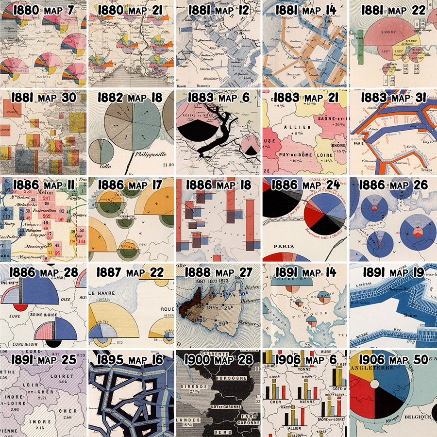
• theme_cheysson_map() - Optimized for cartographic work

These were derived by RJ Andrews from a collection of 25 thematic maps across the span of years in which the Albums were produced, shown below.

From these, he abstracted the following combinations of color and pattern he thought characterized these maps:

New here

This initial version (1.0.1) of the package defined separate functions and ggplot2 scales for color palettes and shading patterns.

Combining them correctly in one plot took real fixing: the pattern scales (scale_pattern_type_cheysson(), scale_pattern_fill_cheysson()) had bugs that silently prevented pattern type and color from varying by category at all - now fixed, so colors and patterns can be layered together as shown below.

A fully unified API that applies Cheysson’s actual designed color-pattern pairings in a single call, matching the combined look of the original Albums, is still in development.

🚀 Quick Start

Here are a few examples to get you started.

Basic Color Palette

Use the color palette of the 1881 Album, plate 4

library(ggplot2)
library(ggCheysson)

ggplot(iris, aes(Sepal.Length, Sepal.Width, color = Species)) +
  geom_point(size = 3) +
  scale_color_cheysson("1881_22") +
  labs(title = "Iris Dataset") +
  theme_minimal()

With Fonts and Theme

# Load Cheysson fonts (once per session)
load_cheysson_fonts(method = "showtext")
# Enable showtext for rendering
showtext::showtext_auto()

p1 <- ggplot(mtcars, aes(wt, mpg, color = factor(cyl))) +
  geom_point(size = 3) +
  scale_color_cheysson("1883_31") +
  labs(
    title = "Automobile Efficiency",
    subtitle = "Weight vs Fuel Economy",
    x = "Weight (1000 lbs)",
    y = "Miles per Gallon"
  )

p1 + theme_cheysson()

Scaling with base_size

Like other ggplot2 themes, theme_cheysson() takes a base_size for larger output (slides, posters). Title and axis-title text (set in the decorative CheyssonTitle/CheyssonSansCaps fonts) is corrected to scale at the same rate as the rest of the theme, rather than reading undersized as base_size grows:

p1 + theme_cheysson(base_size = 14)

p1 + theme_cheysson(base_size = 16)

Complete Cheysson Aesthetic (Colors + Patterns + Fonts)

library(ggpattern)

data <- data.frame(
  category = LETTERS[1:4],
  value = c(15, 23, 18, 20)
)

# Pull the palette's pattern specs directly, so pattern type and hatch
# color follow the actual data rather than a single fixed pattern
patterns <- cheysson_pattern("1883_30")

ggplot(data, aes(category, value, fill = category)) +
  geom_col_pattern(
    aes(
      pattern = category,
      pattern_fill = category,
      pattern_fill2 = category,
      pattern_angle = category
    ),
    pattern_density = 0.35,
    color = "black"
  ) +
  scale_fill_cheysson_pattern("1883_30") +
  scale_pattern_manual(values = cheysson_pattern_params(patterns, "pattern_type")) +
  scale_pattern_fill_manual(values = cheysson_pattern_params(patterns, "pattern_fill")) +
  scale_pattern_fill2_cheysson("1883_30") +
  scale_pattern_angle_cheysson("1883_30") +
  labs(
    title = "Statistical Comparison",
    x = "Category",
    y = "Value"
  ) +
  theme_cheysson() +
  theme(legend.position = "none")

🌈 Available Palettes

cheysson_palettes provides 25 named color palettes, each with its type (sequential, diverging, grouped, or category), the album year and plate number it was extracted from, and its hex color codes.

library(ggCheysson)

# List all palettes
list_cheysson_pals()
#>       name       type album plate n_colors
#> 1  1880_07    grouped  1880     7        5
#> 2  1880_21   category  1880    21        7
#> 3  1881_12 sequential  1881    12        1
#> 4  1881_14    grouped  1881    14        2
#> 5  1881_22   category  1881    22        4
#> 6  1881_30    grouped  1881    30        5
#> 7  1882_18    grouped  1882    18        2
#> 8  1883_21  diverging  1883    21        3
#> 9  1883_30   category  1883    30        4
#> 10 1883_31  diverging  1883    31        2
#> 11 1886_11    grouped  1886    11        4
#> 12 1886_17    grouped  1886    17        3
#> 13 1886_18    grouped  1886    18        3
#> 14 1886_24    grouped  1886    24        3
#> 15 1886_26 sequential  1886    26        2
#> 16 1886_28   category  1886    28        3
#> 17 1887_22    grouped  1887    22        2
#> 18 1888_27 sequential  1888    27        1
#> 19 1891_14    grouped  1891    14        2
#> 20 1891_19 sequential  1891    19        1
#> 21 1891_25 sequential  1891    25        2
#> 22 1895_16 sequential  1895    16        3
#> 23 1900_28 sequential  1900    28        2
#> 24 1906_06   category  1906     6        6
#> 25 1906_50   category  1906    50        4

# List by type
list_cheysson_pals("sequential")
#>      name       type album plate n_colors
#> 1 1881_12 sequential  1881    12        1
#> 2 1886_26 sequential  1886    26        2
#> 3 1888_27 sequential  1888    27        1
#> 4 1891_19 sequential  1891    19        1
#> 5 1891_25 sequential  1891    25        2
#> 6 1895_16 sequential  1895    16        3
#> 7 1900_28 sequential  1900    28        2

# View palette colors
cheysson_pal("1880_21")
#> [1] "#d9636c" "#869e80" "#dec367" "#85aab1" "#aea9a4" "#ed8238" "#ab90a4"

Visualizing Palettes

Use show_palette() to display a palette with color swatches and hex codes:

# Display a single palette with metadata
show_palette("1895_16")

# Display multiple palettes at once
show_palettes(c("1880_21", "1906_06", "1881_30"))

# One palette of each type in a 2x2 grid: category, sequential, diverging, grouped
show_palettes(c("1880_21", "1895_16", "1883_21", "1881_30"), ncol = 2)

Some palettes, such as the sequential 1881_12, have only one color: Cheysson made the steps with hatching of increasing density rather than with shades. Their swatches here show a single color; use cheysson_pattern("1881_12") to get the full palette (see Pattern Support, below).

# Display all palettes of a specific type
show_palettes("category")

Palette types:

• Sequential (7 palettes): For ordered quantitative data
• Diverging (2 palettes): For data with neutral midpoint
• Grouped (10 palettes): For comparing related groups
• Category (6 palettes): For categorical data

📐 Pattern Support

With ggpattern, recreate the distinctive hatching styles - each palette pairs colors with historically accurate patterns (solid fills, stripes, crosshatching):

library(ggpattern)

# List available pattern palettes
head(list_cheysson_patterns())
#>      name       type album plate n_patterns
#> 1 1880_07    grouped  1880     7          7
#> 2 1880_21   category  1880    21          7
#> 3 1881_12 sequential  1881    12          3
#> 4 1881_14    grouped  1881    14          4
#> 5 1881_22   category  1881    22          4
#> 6 1881_30    grouped  1881    30          8

# Get pattern specifications for one palette
patterns <- cheysson_pattern("1886_24")

# Display the palette's patterns as swatches
n <- length(patterns)
ggplot(data.frame(i = factor(seq_len(n))), aes(i, 1, fill = i)) +
  geom_col_pattern(
    aes(pattern = i, pattern_fill = i, pattern_angle = i),
    pattern_density = 0.35, pattern_spacing = 0.03,
    color = "black", width = 0.95
  ) +
  scale_fill_manual(values = cheysson_pattern_params(patterns, "fill")) +
  scale_pattern_fill_manual(values = cheysson_pattern_params(patterns, "pattern_fill")) +
  scale_pattern_manual(values = cheysson_pattern_params(patterns, "pattern_type")) +
  scale_pattern_angle_manual(values = cheysson_pattern_params(patterns, "pattern_angle")) +
  theme_void() +
  theme(legend.position = "none")

Use the pattern scales directly in a plot, alongside the matching fill scale:

data <- data.frame(category = LETTERS[1:4], value = c(15, 23, 18, 20))

ggplot(data, aes(category, value, fill = category)) +
  geom_col_pattern(
    aes(pattern = category, pattern_fill = category),
    pattern_density = 0.35, color = "black"
  ) +

    scale_fill_cheysson_pattern("1886_24") +
  scale_pattern_manual(values = cheysson_pattern_params(patterns, "pattern_type")[1:4]) +
  scale_pattern_fill_manual(values = cheysson_pattern_params(patterns, "pattern_fill")[1:4]) +
  labs(title = "Statistical Comparison", x = "Category", y = "Value") +
  theme_minimal()

✍️ Font Families

Five Cheysson font families are included:

Two of these, CheyssonTitle and CheyssonOutlineCaps are designed to be decorative, mainly used in titles

Here are the others:

To use these:

# Load fonts
load_cheysson_fonts(method = "showtext")
showtext::showtext_auto()

# View font metadata
cheysson_fonts

# Use specific fonts
theme(
  plot.title = element_text(family = "CheyssonTitle"),
  axis.title = element_text(family = "CheyssonSansCaps"),
  axis.text = element_text(family = "Cheysson")
)

📦 Package Contents

Data

• cheysson_palettes - Color palette specifications (25 palettes)
• cheysson_patterns - Pattern/hatching specifications (134 patterns)
• cheysson_fonts - Font family metadata (5 fonts)
• albumImages - Metadata linking palettes to original album plates

Color Functions

• cheysson_pal() - Get colors from a palette
• scale_color_cheysson() / scale_fill_cheysson() - ggplot2 color scales
• list_cheysson_pals() - List available palettes
• show_palette() - Display a single palette with color swatches and hex codes
• show_palettes() - Display multiple palettes for comparison

Pattern Functions

• cheysson_pattern() - Get pattern specifications
• scale_pattern_*_cheysson() - ggpattern scales for fills, types, angles, densities
• list_cheysson_patterns() - List available pattern palettes

Font Functions

• load_cheysson_fonts() - Load font families
• cheysson_font() - Get font family names
• cheysson_fonts_available() - Check font availability

Themes

• theme_cheysson() - Complete Cheysson theme
• theme_cheysson_minimal() - Minimal variant
• theme_cheysson_map() - For maps

🙏 Sources and Attribution

Color Palettes and Patterns

• David Rumsey Map Collection: Complete digitized Albums de Statistique Graphique View collection

• RJ Andrews: SVG pattern extraction and digitization Classic Map Color Design | GitHub

• Tom Shanley: Observable implementation Cheysson Color Palettes

Fonts

• Kenneth Fields: Hand-drawn font family creation The style of Émile Cheysson

🖼️ Gallery

Original maps from the Albums showing the variety of colors and patterns

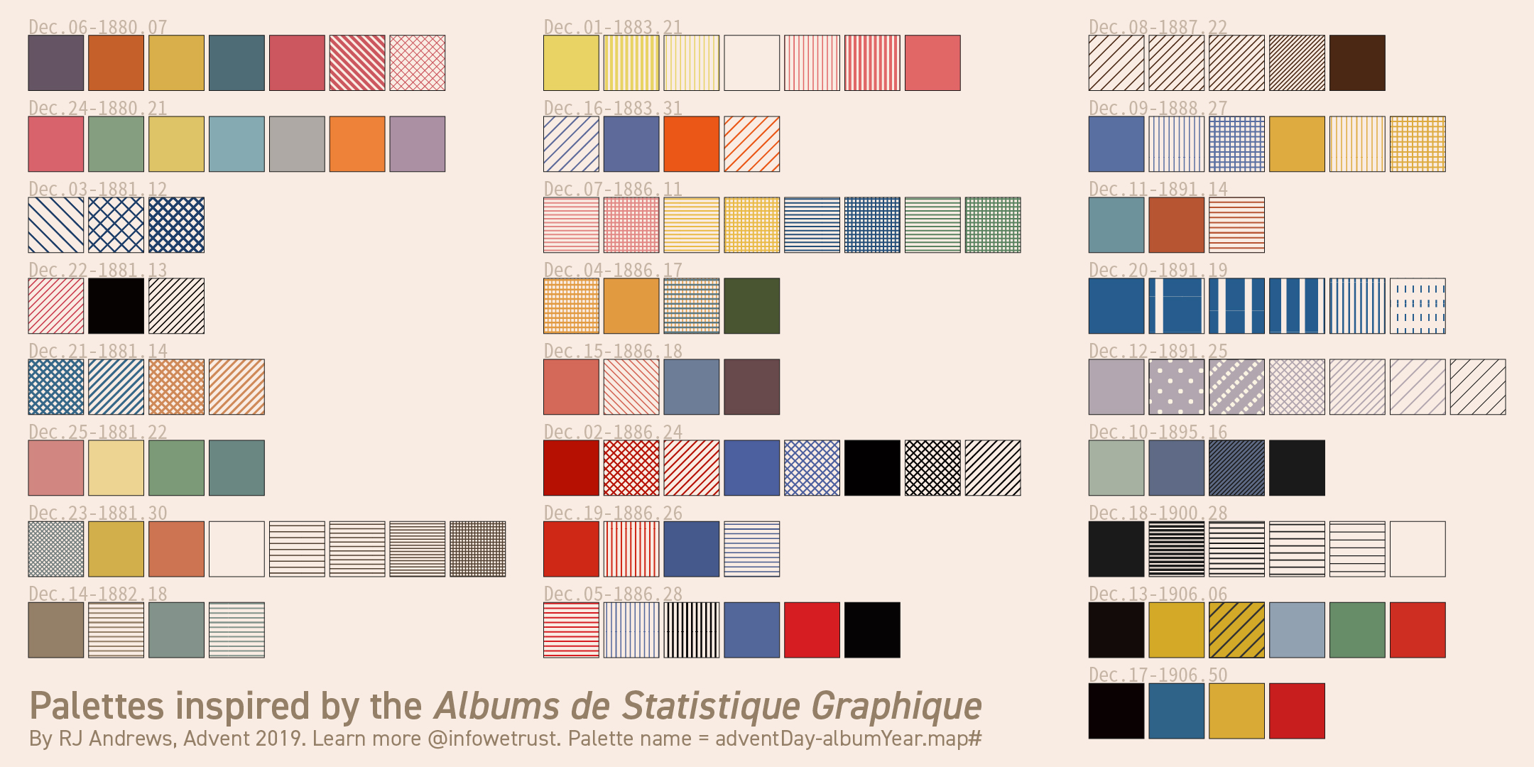
Extracted color palettes by RJ Andrews

🚧 Development Status

This package is under active development. Current features are stable and tested, but the API may evolve. Feedback and contributions are welcome!

🔗 Related Packages

• ggpattern - Pattern fills for ggplot2
• ggthemes - Additional themes for ggplot2
• systemfonts - Font handling for R

⚖️ License

GPL (>= 3)

📖 Citation

To cite ggCheysson, please use:

citation("ggCheysson")
#> To cite package 'ggCheysson' in publications use:
#> 
#>   Friendly M (2026). _ggCheysson: Graphic Styles of Emile Cheysson for
#>   'ggplot2'_. R package version 1.1.0,
#>   <https://github.com/friendly/ggCheysson>.
#> 
#> A BibTeX entry for LaTeX users is
#> 
#>   @Manual{,
#>     title = {ggCheysson: Graphic Styles of Emile Cheysson for 'ggplot2'},
#>     author = {Michael Friendly},
#>     year = {2026},
#>     note = {R package version 1.1.0},
#>     url = {https://github.com/friendly/ggCheysson},
#>   }

To cite the original Albums de Statistique Graphique:

France. Ministère des travaux publics. Album de statistique graphique de [year]. Paris: Imprimerie nationale, [1879-1897].

📚 References

Friendly, M. (2008). The Golden Age of Statistical Graphics. Statistical Science, 23(4), 502–535. https://doi.org/10.1214/08-STS268