
Constrained Delaunay triangulation with refinement for R, binding the header-only CDT library (MPL-2.0). It takes the same input as a planar straight line graph (vertices, segments as index pairs, optional per-vertex attributes) and returns vertices, triangles, and a per-triangle depth that says where each triangle sits relative to the constraints, with no point-in-polygon step.
remotes::install_github("hypertidy/cdtr")Vertices and segments in, vertices and triangles out. Here a square with a square hole: two closed rings of segments.
library(cdtr)
x <- c(0, 1, 1, 0, 0.25, 0.75, 0.75, 0.25)
y <- c(0, 0, 1, 1, 0.25, 0.25, 0.75, 0.75)
s0 <- 1:8; s1 <- c(2, 3, 4, 1, 6, 7, 8, 5)
r <- cdt_triangulate(x, y, s0, s1)
str(r[c("P", "T", "S", "depth")])
#> List of 4
#>  $ P    : num [1:8, 1:2] 0 1 1 0 0.25 0.75 0.75 0.25 0 0 ...
#>  $ T    : int [1:10, 1:3] 8 6 8 7 6 5 8 6 2 2 ...
#>  $ S    : int [1:8, 1:2] 1 3 1 5 6 2 7 5 2 4 ...
#>  $ depth: int [1:10] 2 1 1 1 2 1 1 1 1 1
depth is the number of constraint boundaries crossed on
the way in from outside: 0 is outside everything, and for nested rings
odd is inside, even is a hole. By default triangles outside the
outermost boundary are already dropped (erase = "outer",
which is what Triangle’s -p does);
erase = "holes" also drops the even depths.
plot_mesh <- function(m, main = "") {
  e <- cdt_edges(m)
  plot(m$P, asp = 1, axes = FALSE, xlab = "", ylab = "", pch = ".", main = main)
  segments(m$P[e[, 1], 1], m$P[e[, 1], 2], m$P[e[, 2], 1], m$P[e[, 2], 2], col = "grey50")
  segments(m$P[m$S[, 1], 1], m$P[m$S[, 1], 2], m$P[m$S[, 2], 1], m$P[m$S[, 2], 2], lwd = 2)
}
op <- par(mfrow = c(1, 3), mar = c(0.5, 0.5, 2, 0.5))
plot_mesh(r, "constrained")
plot_mesh(cdt_triangulate(x, y, s0, s1, max_area = 0.01), "max_area = 0.01")
plot_mesh(cdt_triangulate(x, y, s0, s1, max_area = 0.01, min_angle = 25, erase = "holes"),
          "+ min_angle = 25, holes erased")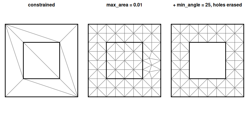
par(op)Ruppert refinement cannot always meet the bound (two constraints meeting at a sharp angle, say). Rather than silently stopping, the result carries the counts.
r2 <- cdt_triangulate(x, y, s0, s1, max_area = 0.01, min_angle = 25)
r2$unrefined
#>   criterion shortEdgeTriangles circumcenterOutside circumcenterOnVertex
#> 1      area                  0                   0                    0
#> 2     angle                  0                   0                    0
#>   sharpFixedCorner shortEdges splitVertexInvalid
#> 1                0          0                  0
#> 2                0          0                  0
r2$min_edge_length
#> [1] 0.025
min_edge_length is the floor below which the refiner
gives up on an edge; by default it is derived from the input (a fraction
of the median segment length, capped by the area target) so refinement
does not cascade into sharp input corners. Pass 0 for
never-give-up.
Refinement follows Ruppert’s algorithm: a constraint segment is split
whenever a vertex lies inside the circle on its diameter, and this
applies to max_area alone as well as to
min_angle. So a mesh refined by area has more vertices
along the constraints than one from a refiner that only splits large
triangles (Triangle with a but no q, for
example). With max_area set to 1/5000 of the bounding box
area, on North Carolina’s counties and anglr’s Tasmanian cadastre and
contours, cdtr adds 1.2 to 1.3 times as many Steiner vertices as
Triangle with a alone, and 40 to 62% of them lie on the
input constraints, against 11 to 14% of Triangle’s. On the two polygon
layers that buys shape: 0.1% of cdtr’s triangles have a minimum angle
under 5 degrees on the counties, against 0.6% of Triangle’s, and 1.7%
against 3.0% on the cadastre. On the contours the share is the same,
1.4%. These figures come from inst/benchmarks/bench5.R.
min_edge_length is the control. Edges shorter than it
are not split, so a larger value gives a coarser mesh. By default it is
derived from the input (2.8 on the contours, where
sqrt(max_area) is 12). On these three inputs a floor of
sqrt(max_area) cuts cdtr’s Steiner vertices by 10 to 12%,
and the area target is still met everywhere on the two polygon layers.
Raise it in steps, and check unrefined and the largest
triangle area each time.
erase = "holes" drops the even depths. A hole can also
be given as a point, as the H of an
RTriangle::pslg(): the region around it that is bounded by
segments is erased, whatever its depth.
rh <- cdt_triangulate(x, y, s0, s1, holes = cbind(0.5, 0.5))
table(rh$depth)
#>
#> 1
#> 8Any polygon source reduces to the same two tables. With
sf’s North Carolina counties, rings become vertex runs and
consecutive index pairs; shared boundaries dedupe to one segment.
nc <- sf::st_read(system.file("shape/nc.shp", package = "sf"), quiet = TRUE)
rings <- unlist(lapply(sf::st_geometry(nc), function(g) lapply(unclass(g), `[[`, 1)), recursive = FALSE)
xy <- do.call(rbind, lapply(rings, function(m) m[-nrow(m), ]))
n <- vapply(rings, function(m) nrow(m) - 1L, 1L)
start <- rep(cumsum(c(0L, n[-length(n)])), n)
s0 <- seq_along(xy[, 1])
s1 <- start + (s0 - start) %% rep(n, n) + 1L
m <- cdt_triangulate(xy[, 1], xy[, 2], s0, s1, max_area = 0.01)
table(m$depth)
#>
#>    1    3    5
#> 2100 1119  521
op <- par(mar = rep(0, 4))
plot_mesh(m)
par(op)The counties tile the state, so there are no holes, but a county two boundaries in from the coast has depth 3, and so on: depth is the peel layer, a count of constraint crossings from outside, not an inside/outside flag in general. It is computed topologically from the mesh alone, before anything is erased, which makes it a cheap first cut for classifying triangles by region: nested rings get odd/even, a coverage gets a boundary-distance ordering, and only ties within a layer need a geometric lookup.
Per-vertex values (an elevation, a time) are carried onto the new
Steiner vertices by linear interpolation from the input mesh, the way
Triangle’s PA works.
z <- 2 * xy[, 1] + 3 * xy[, 2]
ma <- cdt_triangulate_attr(xy[, 1], xy[, 2], s0, s1, PA = cbind(z = z), max_area = 0.01)
range(ma$PA[, "z"] - (2 * ma$P[, 1] + 3 * ma$P[, 2]))
#> [1] -1.421085e-14 1.421085e-14cdt_quality() gives the shape of every triangle: area,
angles, edge lengths and radius-edge ratio.
summary(cdt_quality(m)[c("area", "min_angle", "radius_edge")])
#>       area             min_angle       radius_edge
#>  Min.   :6.430e-06   Min.   : 2.546   Min.   : 0.5778
#>  1st Qu.:8.159e-04   1st Qu.:21.217   1st Qu.: 0.7234
#>  Median :2.977e-03   Median :33.813   Median : 0.8985
#>  Mean   :3.376e-03   Mean   :32.666   Mean   : 1.2297
#>  3rd Qu.:5.462e-03   3rd Qu.:43.721   3rd Qu.: 1.3816
#> Max. :9.997e-03 Max. :59.931 Max. :11.2560cdt_locate() finds the triangle holding each query point
with exact orientation tests, so a point on a shared edge is never lost
between triangles. With barycentric = TRUE it also gives
the weights of the triangle’s vertices at each point.
cdt_locate(m$P, m$T, c(-80, -79), c(35.5, 35.5), barycentric = TRUE)
#>   triangle        b1        b2         b3
#> 1     1225 0.3858433 0.5537999 0.06035678
#> 2 379 0.1891296 0.7195179 0.09135246edge_sources = TRUE returns, for every fixed edge, the
input segments that cover it (through crossings, splits and refinement).
That lets regions be labelled by which inputs cover them, which
depth cannot do, and cdt_winding() uses it to
give the winding number of each input feature in every triangle, for
overlapping polygons, with no point-in-polygon test. See
vignette("overlay").
The wkpool package
(0.5.0 and later) reads any geometry that ‘wk’ handles, shares
coincident vertices, and uses cdtr for the constrained triangulation
behind tri_overlay() and tri_overlay_relate().
The output of cdt_pslg() goes straight into
wkpool::new_wkpool_tri(), as shown in
vignette("wkpool", package = "cdtr"). The polymer package builds
many-layer polygon overlay on both.
vignette("cdtr"): a tour of the package.vignette("wkpool"): polygons, triangle pools and
wkpool.vignette("terrain"): a surface from contour lines, and
how triangle quality relates to its error.vignette("overlay"): overlapping inputs,
edge_sources and cdt_winding().cdtr is the builds-anywhere, permissively licensed
baseline of the hypertidy meshing stack, and the triangulation behind
its polygon overlay tools. It has value on its own: what it adds to a
triangulation is information about how the mesh relates to its input,
namely region depth, vertex origin, the input segments behind every
constraint edge, and per-feature winding.
It shares a vertices, segments and triangles contract with other
backends, so which one to use is a choice and not a rewrite. RTriangle
(Shewchuk’s Triangle) is the established one in R, and
cdt_pslg() accepts its pslg input as it is. laridae provides CGAL’s
constrained triangulations and meshing, as a persistent mesh that can be
edited and refined. Having more than one option opens up more of what
can be done with triangulation in R.
The inst/benchmarks/ scripts compare cdtr and RTriangle
on North Carolina’s counties and anglr’s Tasmanian cadastre, which are
polygons, and its Tasmanian contours, which are open lines and are
meshed over their convex hull (the scripts need anglr, which is no
longer on CRAN). Constrained-only, the two give meshes of the same size,
with the same largest area and smallest angle, on all three. With
max_area both meet the target on the polygons. Over the
hull of the contours cdtr leaves 0.3% of triangles above it, and reports
them in unrefined as circumcenterOutside. cdtr
adds more Steiner vertices (on the contours, 5,835 against 5,343
vertices in total), because it protects the constraints (see above), and
reports in unrefined where it declined to refine. Its
smallest angles are better on the counties but equally poor on the
contours. Triangle is faster: about three times on the counties with
refinement, and about one and a half times on the cadastre without (the
timings in bench.R, on one machine), so it is the better
choice if speed on a large problem matters more than the extra
features.
Please note that the cdtr project is released with a Contributor Code of Conduct. By contributing to this project, you agree to abide by its terms.